> For the complete documentation index, see [llms.txt](https://www.mlcompendium.com/llms.txt). Markdown versions of documentation pages are available by appending `.md` to page URLs; this page is available as [Markdown](https://www.mlcompendium.com/machine-learning/linear-separator-algorithms.md).
# Linear Separator Algorithms
### **SEQUENTIAL MINIMAL OPTIMIZATION (SMO)**
[**What is the SMO (SVM) classifier?**](https://www.microsoft.com/en-us/research/publication/sequential-minimal-optimization-a-fast-algorithm-for-training-support-vector-machines/?from=http%3A%2F%2Fresearch.microsoft.com%2Fpubs%2F69644%2Ftr-98-14.pdf) **- Sequential Minimal Optimization, or SMO. Training a support vector machine requires the solution of a very large quadratic programming (QP) optimization problem. SMO breaks this large QP problem into a series of the smallest possible QP problems. These small QP problems are solved analytically, which avoids using a time-consuming numerical QP optimization as an inner loop. The amount of memory required for SMO is linear in the training set size, which allows SMO to handle very large training sets. Because matrix computation is avoided, SMO scales somewhere between linear and quadratic in the training set size for various test problems, while the standard chunking SVM algorithm scales somewhere between linear and cubic in the training set size. SMO’s computation time is dominated by SVM evaluation, hence SMO is fastest for linear SVMs and sparse data sets. On real-world sparse data sets, SMO can be more than 1000 times faster than the chunking algorithm.**
[**Differences between libsvm and liblinear**](https://stackoverflow.com/questions/11508788/whats-the-difference-between-libsvm-and-liblinear) **&** [**smo vs libsvm**](https://stackoverflow.com/questions/23674411/weka-smo-vs-libsvm)
### **SUPPORT VECTOR MACHINES (SVM)**
**-** [**Definition**](http://docs.opencv.org/3.0-beta/modules/ml/doc/support_vector_machines.html)**,** [**tutorial**](https://jakevdp.github.io/PythonDataScienceHandbook/05.07-support-vector-machines.html)**\*\*\*:**
* **For Optimal 2-class classifier.**
* **Extended for regression and clustering problems (1 class).**
* **Kernel-based**
* **maps feature vectors into a higher-dimensional space using a kernel function**
* **builds an optimal linear discriminating function in this space (linear?) or an optimal hyper-plane (RBF?) that fits the training data**
* **In case of SVM, the kernel is not defined explicitly.**
* **A distance needs to be defined between any 2 points in the hyper-space.**
* **The solution is optimal, the margin is maximal. between the separating hyper-plane and the nearest feature vectors**
* **The feature vectors that are the closest to the hyper-plane are called support vectors, which means that the position of other vectors does not affect the hyper-plane (the decision function).**
* **The model produced by support vector classification (as described above) depends only on a subset of the training data, because the cost function for building the model does not care about training points that lie beyond the margin.**
### [**MULTI CLASS SVM**](https://www.csie.ntu.edu.tw/~cjlin/papers/multisvm.pdf)
[ ](https://www.csie.ntu.edu.tw/~cjlin/papers/multisvm.pdf)**- one against all, one against one, and Direct Acyclic Graph SVM (one against one with DAG). bottom line One Against One in LIBSVM.**
[**A few good explanation about SVM, formulas, figures, C, gamma, etc.**](https://www.quora.com/What-are-C-and-gamma-with-regards-to-a-support-vector-machine)
**Math of SVM on youtube:**
* [**very good number-based example #1**](https://www.youtube.com/watch?v=1NxnPkZM9bc)
* [**Very good but lengthy and chatty example with make-sense math #2**](https://www.youtube.com/watch?v=mU_N3nmv0Go\&list=PLAwxTw4SYaPlkESDcHD-0oqVx5sAIgz7O\&index=4) **- udacity**
* **Linear - maximize the margin, optimal solution, only a few close points are really needed the others are zeroes by the alphas (alpha says “pay attention to this variable”) in the quadratic programming equation. XtX is a similarity function (pairs of points that relate to each other in output labels and how similar to one another, Xi’s point in the same direction) y1y2 are the labels. Therefore further points are not needed. But the similarity is important here(?)**
* **Non-linear - e.g. circle inside a circle, needs to map to a higher plane, a measure of similarity as XtX is important. We use this similarity idea to map into a higher plane, but we choose the higher plane for the purpose of a final function that behaves likes a known function, such as (A+B)^2. It turns out that (q1,q2,root(2)q1q2) is engineered with that root(2) thing for the purpose of making the multiplication of X^tY, which turns out to be (X^tY)^2. We can substitute this formula (X^tY)^2 instead of the X^tX in the quadratic equation to do that for us.This is the kernel trick that maps the inner class to one side and the outer circle class to the other and passes a plane in between them.**
* **Similarity is defined intuitively as all the points in one class vs the other.. I think**
* **A general kernel K=(X^tY + C)^p is a polynomial kernel that can define the above function and others.**
* **Quadratic eq with possible kernels including the polynomial.**
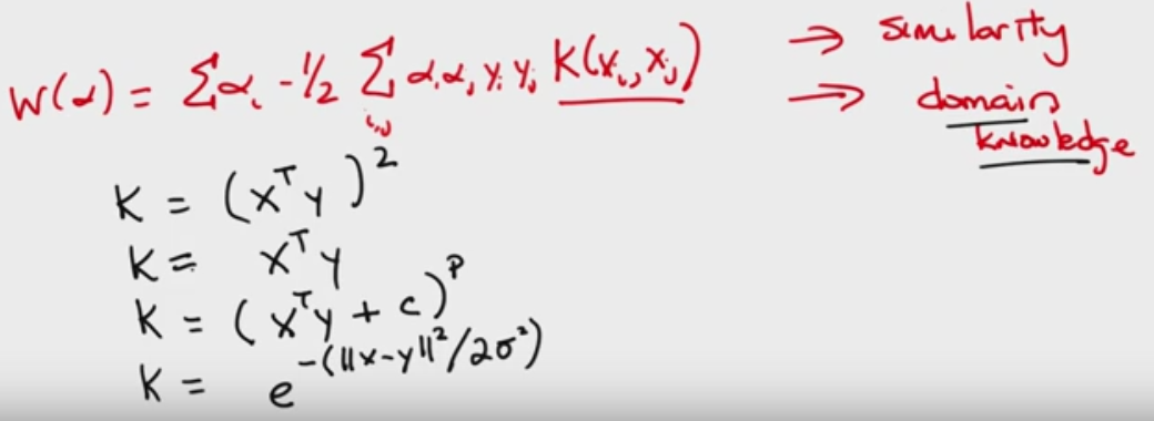
* **Most importantly the kernel function is our domain knowledge. (?) IMO we should choose a kernel that fits our feature data.**
* **The output of K is a number(?)**
* **Infinite dimensions - possible as well.**
* **Mercer condition - it acts like a distance\similar so that is the “rule” of which a kernel needs to follow.**
* [**Super good lecture on MIT OPEN COURSE WARE**](https://www.youtube.com/watch?v=_PwhiWxHK8o) **- expands on the quadratic equations that were introduced in the previous course above.**
### **Regularization and influence**
**- (basically punishment for overfitting and raising the non- linear class points higher and lower)**
* [**How does regularization look like in SVM**](https://datascience.stackexchange.com/questions/4943/intuition-for-the-regularization-parameter-in-svm) **- controlling ‘C’**
* [**The best explanation about Gamma (and C) in SVM!**](https://www.quora.com/What-are-C-and-gamma-with-regards-to-a-support-vector-machine)
### **SUPPORT VECTOR REGRESSION (SVR)**
**-** [**Definition Support Vector Regression**](http://scikit-learn.org/stable/modules/svm.html#svm-implementation-details)**.:**
* **The method of SVM can be extended to solve regression problems.**
* **Similar to SVM, the model produced by Support Vector Regression depends only on a subset of the training data, because the cost function for building the model ignores any training data close to the model prediction.**
### [**LibSVM vs LibLinear**](https://stackoverflow.com/questions/11508788/whats-the-difference-between-libsvm-and-liblinear)
**- using many kernel transforms to turn a non-linear problem into a linear problem beforehand.**
**From the link above, it seems like liblinear is very much the same thing, without those kernel transforms. So, as they say, in cases where the kernel transforms are not needed (they mention document classification), it will be faster.**
* **libsvm (SMO) implementation**
* **kernel (n^2)**
* **Linear SVM (n^3)**
* **liblinear - optimized to deal with linear classification without kernels**
* **Complexity O(n)**
* **does not support kernel SVMs.**
* **Scores higher**
**n is the number of samples in the training dataset.**
**Conclusion: In practice libsvm becomes painfully slow at 10k samples. Hence for medium to large scale datasets use liblinear and forget about libsvm (or maybe have a look at approximate kernel SVM solvers such as** [**LaSVM**](http://leon.bottou.org/projects/lasvm)**, which saves training time and memory usage for large scale datasets).**
### **Support vector clustering (SVC)**
[**paper**](http://www.jmlr.org/papers/volume2/horn01a/horn01a.pdf)**,** [**short explanation**](https://www.quora.com/Is-it-possible-to-use-SVMs-for-unsupervised-learning-density-estimation)
### **KERNELS**
[**What are kernels in SVM**](https://www.quora.com/What-are-Kernels-in-Machine-Learning-and-SVM) **- intuition and example**
* **allows us to do certain calculations faster which otherwise would involve computations in higher dimensional space.**
* **K(x, y) = \. Here K is the kernel function, x, y are n dimensional inputs. f is a map from n-dimension to m-dimension space. < x,y> denotes the dot product. usually m is much larger than n.**
* **normally calculating \ requires us to calculate f(x), f(y) first, and then do the dot product. These two computation steps can be quite expensive as they involve manipulations in m dimensional space, where m can be a large number.**
* **Result is ONLY a scalar, i..e., 1-dim space.**
* **We don’t need to do that calc if we use a clever kernel.**
**Example:**
**Simple Example: x = (x1, x2, x3); y = (y1, y2, y3). Then for the function f(x) = (x1x1, x1x2, x1x3, x2x1, x2x2, x2x3, x3x1, x3x2, x3x3), the kernel is K(x, y ) = (\)^2.**
**Let's plug in some numbers to make this more intuitive: suppose x = (1, 2, 3); y = (4, 5, 6). Then:**
**f(x) = (1, 2, 3, 2, 4, 6, 3, 6, 9) and f(y) = (16, 20, 24, 20, 25, 30, 24, 30, 36)**
**\ = 16 + 40 + 72 + 40 + 100+ 180 + 72 + 180 + 324 = 1024 i.e., 1\*16+2\*20+\*3\*24..**
**A lot of algebra. Mainly because f is a mapping from 3-dimensional to 9 dimensional space.**
**With a kernel its faster.**
**K(x, y) = (4 + 10 + 18 ) ^2 = 32^2 = 1024**
**A kernel is a magical shortcut to calculate even infinite dimensions!**
[**Relation to SVM**](https://www.quora.com/What-are-Kernels-in-Machine-Learning-and-SVM)**?:**
* **The idea of SVM is that y = w phi(x) +b, where w is the weight, phi is the feature vector, and b is the bias.**
* **if y> 0, then we classify datum to class 1, else to class 0.**
* **We want to find a set of weight and bias such that the margin is maximized.**
* **Previous answers mention that kernel makes data linearly separable for SVM. I think a more precise way to put this is, kernels do not make the the data linearly separable.**
* **The feature vector phi(x) makes the data linearly separable. Kernel is to make the calculation process faster and easier, especially when the feature vector phi is of very high dimension (for example, x1, x2, x3, ..., x\_D^n, x1^2, x2^2, ...., x\_D^2).**
* **Why it can also be understood as a measure of similarity: if we put the definition of kernel above, \, in the context of SVM and feature vectors, it becomes \. The inner product means the projection of phi(x) onto phi(y). or colloquially, how much overlap do x and y have in their feature space. In other words, how similar they are.**
[**Kernels**](http://docs.opencv.org/3.0-beta/modules/ml/doc/support_vector_machines.html)**:**
* **SVM::LINEAR Linear kernel. No mapping is done, linear discrimination (or regression) is done in the original feature space. It is the fastest option.** 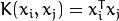**.**
* **SVM::RBF Radial basis function (RBF), a good choice in most cases.** 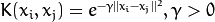**.**
### [**Intuition for regularization in SVM**](https://datascience.stackexchange.com/questions/4943/intuition-for-the-regularization-parameter-in-svm)
[**Grid search for SVM Hyper parameters**](http://docs.opencv.org/3.0-beta/modules/ml/doc/support_vector_machines.html) **- in openCV.** [**Example in log space**](https://stackoverflow.com/questions/29128074/choosing-the-best-svm-kernel-type-and-parameters-using-opencv-on-python)
* [**I.e., (for example**](https://www.csie.ntu.edu.tw/~cjlin/papers/guide/guide.pdf)**, C = 2^-5 , 2 ^-3 , . . . , 2^15 , γ = 2^-15 , 2 ^-13 , . . . , 2^3 ).**
* **There are heuristic methods that skip some search options**
* **However, no need for heuristics, computation-time is small, grid can be paralleled and we dont skip parameters.**
* **Controlling search complexity using two tier grid, coarse grid and then fine tune.**
### [**Overfitting advice for SVM:** ](https://stats.stackexchange.com/questions/35276/svm-overfitting-curse-of-dimensionality)
* **Regularization parameter C -** [**penalty example**](http://scikit-learn.org/stable/auto_examples/svm/plot_rbf_parameters.html)
* **In non linear kernels:**
* **Kernel choice**
* **Kernel parameters**
* [**RBF**](http://scikit-learn.org/stable/auto_examples/svm/plot_rbf_parameters.html) **- gamma, low and high values are far and near influence**
* **Great** [**Tutorial at LIBSVM**](https://www.csie.ntu.edu.tw/~cjlin/papers/guide/guide.pdf)
* **Reasonable first choice**
* **when the relation between class labels and attributes is nonlinear.**
* **Special case of C can make this similar to linear kernel (only! After finding C and gamma)**
* **Certain parameters makes it behave like the sigmoid kernel.**
* **Less hyperparameters than RBF kernel.**
* **0 \> number of features. Usually high dimensional mapping using non linear kernel. If we insist on liblinear, -s 2 leads to faster training.**
[**Kdnuggets: When to use DL over SVM and other algorithms. Computationally expensive for a very small boost in accuracy.**](http://www.kdnuggets.com/2016/04/deep-learning-vs-svm-random-forest.html)
---
# Agent Instructions
This documentation is published with GitBook. GitBook is the documentation platform designed so that both humans and AI agents can read, navigate, and reason over technical content effectively. Learn more at gitbook.com.
## Querying This Documentation
If you need additional information that is not directly available in this page, you can query the documentation dynamically by asking a question.
Perform an HTTP GET request on the current page URL with the `ask` query parameter:
```
GET https://www.mlcompendium.com/machine-learning/linear-separator-algorithms.md?ask=
```
The question should be specific, self-contained, and written in natural language.
The response will contain a direct answer to the question and relevant excerpts and sources from the documentation.
Use this mechanism when the answer is not explicitly present in the current page, you need clarification or additional context, or you want to retrieve related documentation sections.